As it was said in the previous post, a first step in the relief construction is to obtain the base heights values. Such value at a rhomb point should be derived from global heights grid nodes by the process of averaging. A simple averaging with weights depending on the distance to the nodes will not be enough to obtain a smooth surface, but for some points of rhombs this approach is quite acceptable.

This is true for points on borders of the rhomb when both ends of it are below sea water level. At the moment, there is no goal to make a believable relief of the ocean depths, so we can simply fix values in the points of such borders on the line connecting corresponding nodes of the base heights grid.

In addition, we should do fixing of riverbed points. The value in a riverbed point is made by the averaging values of the surrounding nodes of the global heights grid. So far, this leads to notable stair-stepping effect of the riverbeds, but in general this affects the relief only a little.

According to the above, we can consider the base heights surface as an imaginary surface on which the water of rivers flows into the ocean.

For further explanation I will first resort to a 2D analogy, and then generalize to 3D, illustrating both cases with figures.

Note that in each rhomb there is at least one river, and on continent edges there are also underwater rhomb borders. That is, we always have fixed values in some points in each of land rhombs. From these fixed values we will have to make values in all the other points of the rhomb.

For the 2D case we consider some vertical plane cut crossing two riverbeds (or underwater rhomb borders). Points where riverbeds reside are fixed value points (gray points on figures). And they are usually lie on different elevation levels. A simple approach suggests to make values in intermediate points laying on the connection line of the fixed values.

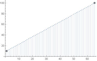
But such approach will inevitably leads to the fact that many rivers will be higher than the surrounding terrain, especially in mountainous areas.

More appropriate approach is the distribution of values as in the following figure.

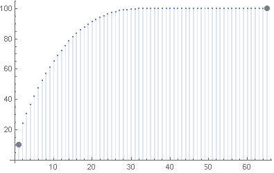
The proposed method of constructing such a distribution of values has the following advantages: the calculation at each point is carried out only once, and you only need to know the distance to one nearest point with a fixed value.

For start, we do the preliminary construction. For each intermediate point we find the nearest fixed value point and assign to the point a pair (d, h), where d is the distance to the nearest fixed point, and h is the value in this fixed point. Next, we sort all points, firstly, by decreasing d and, secondarily, by increasing h. All points together with these pairs form a one-dimensional ordered array A. Subsequently, we will do changes in array A by changing h values without modifying d, and we will not need to do another sorting of the array A.

Further, at each point we calculate the value z = minH + D×(maxH−minH), where maxH and minH are, respectively, the maximum and minimum values of h for points around the current point. We compare the value z with the current value of h at the point. If h<=z, then we set the point new value to z, otherwise we set the value to maxH−1/(d+1)×(maxH−minH). Here, D = min(C×d/(d+1), 1), and C is a coefficient that helps make the curve more convex. In practice, it makes sense to set it to (l+1)/l, where l is half of the rhomb linear size.

Optionally, we may also apply a simple smoothing by the nearest neighbors averaging. In the figure above you see an already smoothed version.

To take into account possible borders of rhombs between rivers, we consider all the rhombs in a certain order (for example, from south to north). We make base heights calculation firstly in the southernmost rhombs, after which the adjacent borders of next rhombs is already considered to be filled with fixed values for subsequent calculations. This process should be continued to the northernmost rhombs.

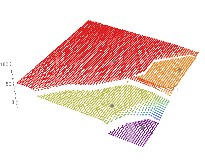
Now we turn to the 3D case and try to apply the same method. For modeling, we consider a variant with several fixed points anywhere in a rhomb. The following figure shows a scheme with fixed value points and a surface composed of distances from a given point to the nearest point with fixed value.

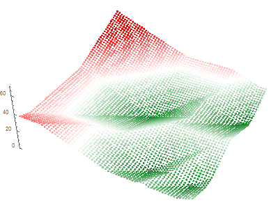
Although, this model does not fully correspond to the real situation with extended rivers in a rhomb, but the nature of the resulting surface and possible problems are the same.

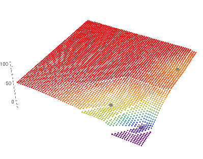
As you can see, the initial surface has gaps. To reduce them, we will should use the same method iteratively, but in every next iteration we must reverse the order of array A. This is what happens if we apply the second iteration.

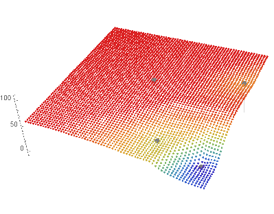
It can be seen that the surface gaps have decreased. Let’s apply the third iteration.

The gaps have become smaller, but still noticeable.

Here, instead of one or more iterations, we can use simple smoothing and get a satisfactory result.

The required number of iterations depends on the initial spread of fixed values. In the project, this iterative process has not yet been fully implemented (only one iteration is done), and the discontinuities of the base heights surface are expressed in oblong and brace-like features in the relief.

The gaps are a consequence of the imperfection of array sorting in favor of the simplicity of calculations at a point. They appear in places of accumulation of values with the same (d, h) pairs. You might think that shuffling points with the same pairs (d, h) can help in reducing iterations, but this only leads to a change in the form of gaps to a less linear, and the convergence does not improve. The limit surface remains nearly the same.

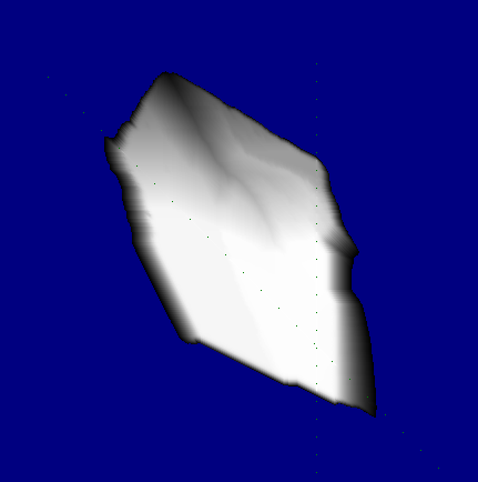
Here is the base heights surface of a small continent, obtained by the project debugging tool. Noticeable surface gaps are clearly visible in the upper-right part. Green dotted lines are the borders of rhombs.

To be continued..