In reality, if we look at satellite images, then we will see a gradual change in the color of the Earth’s surface as a biome changes to another biome. That is, biomes succeed each other gradually, and natural elements of different biomes can be present in the same place at the same time. For example, the vegetation of the subtropics and the vegetation of the temperate zone can be in one place. Although the glacier and the tundra as well as the forest and the steppe have distinct borders.
Nevertheless, for various applications, it’s more convenient to always have distinct borders between zones. And theses borders could be distinguished as separate entities, represented as vector data. The biomes gradient transition on image representations, in principle, should be implemented using styles (although, at the moment I don’t know an appropriate tool somewhere in any GIS).
True Biome Shapes
The creation of true biome shapes occurs in each rhomb separately. First of all, we must take into account values at the points of the global biome shapes, which are located at the vertices of a rhomb.
In the case when all the vertices have the same biome value, we consider that the whole rhomb filled up with this biome.
If the rhomb has from two to four different biomes in its vertices, then we divide the rhomb into two equilateral triangles (upper and lower). To those triangles where biomes at the vertices are different we apply a special mixing method, which I will describe below. It gives a particular picture of biomes when they partially penetrate each other, forming isolated areas, and gradually become solid when increasing distance from the main dividing border.
This mixing method is applied as to the global shapes of biomes in order to mix large areas of biomes, as to the true shapes of biomes defined at the rhombs’ level. On the Serpento, global shapes mixing manifests itself not so often, due to the choice of a too narrow mixing zone, but the true shapes mixing is clearly visible.
Thus, a ‘blurred’ borders are formed. At the moment, with the maximum width in the size of one rhomb.
Mixing method
Here is a description of the method applicable to the square lattice. The project uses a triangular lattice and the application of this method is somewhat more complicated. Moreover, the use of the triangular lattice is rather an exception, the majority of applications which use textures utilize square lattices.
Also, for simplicity, we will restrict ourselves to the case of two biomes. For distinctness, we assume that in the upper vertices of the square is the first biome (with bId=1), and in the lower vertices is the second biome (with bId=2). These values must be determined in advance in the process of building the global biome shapes.
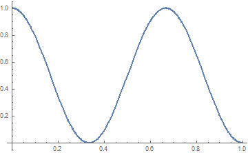
For further, we need the following function, defined on the segment [0, a] (further we assume a=1):
u(y) = -k*atan(s*(y-a/2)) + 0.5, where k = 0.5/atan(s*a/2).
Here, the ‘shrink’ parameter s>=1 allows us to adjust the shape of the resulting curve, and, as a consequence, the possible spread of values. Here are some u(y) function graphics for various s values.
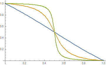
A value of s=1 turns graphic into a straight line.
Now we fill up the square with initial values. To do this, we introduce a Cartesian coordinate system with the horizontal axis x and vertical y, with the origin on the bottom edge of the square (for us it doesn’t matter now where exactly on the bottom edge). Also, we assume that the points on the upper edge have the coordinate y=1.
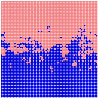
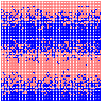
For each point with coordinates (x, y) we calculate the random value r in the interval (0,1). Then we compare the obtained value r with the value u(y) at this point. We set the biome with bId=1 at this point if r>=u(y), and biome with bId=2 otherwise. We get the distribution of biomes similar to which is shown in the following figure (here, s=5).
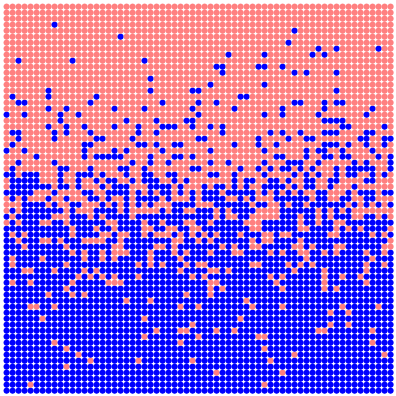
Such a border, although it possesses the property wanted by us, is too chaotic.
To improve it, we can apply a special consolidation process, using a technique similar to that used to construct fractal surfaces with the middle displacement method. To do this, we gradually go through all the points of the square lattice according to the following order. At each step, starting from m=1, we obtain a group of points derivable differently depending on the parity or oddness of m.
- For odd m: all points (1+step+2*step*i, 1+step+2*step*j), where n=2^((m-1)/2), step=1/(2*n), i∈[0..n-1], j∈[0..n-1].
- For even m: all points (1+step*i, 1+step*j), for which i+j is odd, n=2^(m/2), step=1/n, i∈[0..n], j∈[0..n].
For further, it is more convenient for us to go to integer coordinates, where the unit of measurement is the minimum distance between the points, and the square’s edge size ln is equal to the number of edge’s points minus one.
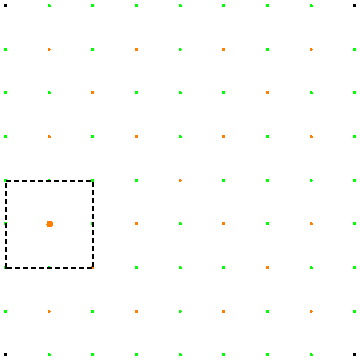
At each point with integer coordinates (i,j) (defined as above for step m), we can determine four origin points (their integer coordinates) from those that have been defined in the previous steps.
- For odd m: {(i-s,j-s), (i-s,j+s), (i+s,j+s), (i+s,j-s)}, where n=2^((m-1)/2), s=ln/(2*n).
- For even m: those points from {{i-s,j}, {i,j-s}, {i+s,j}, {i,j+s}} which lie on the square, n=2^(m/2), s=ln/n
.
Let c1 and c2 are the numbers of origin points of the first and the second biomes. Here, we can define function cf(bId0, c1, c2), which determine the resulting biome at the point from origin points’ biomes and point’s initial biome bId0.
For example, if a function defined as
cf(bId0, c1, c2) = {
    c1>c2: 1,
    c1<c2: 2,
    otherwise: bId0
},
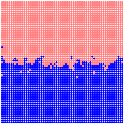
then we obtain the diagram
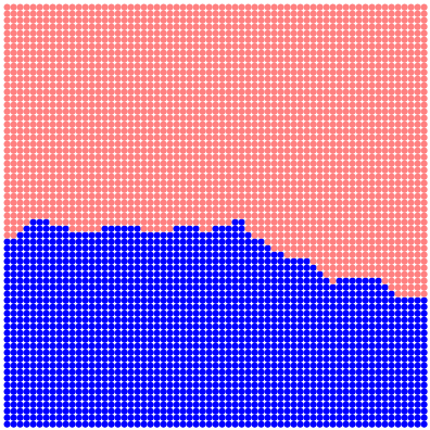
Although this border looks like a fractal, there is no mutual penetration of biomes. Other possible functions of c1 and c2 lead to interesting, but not suitable for us diagrams.
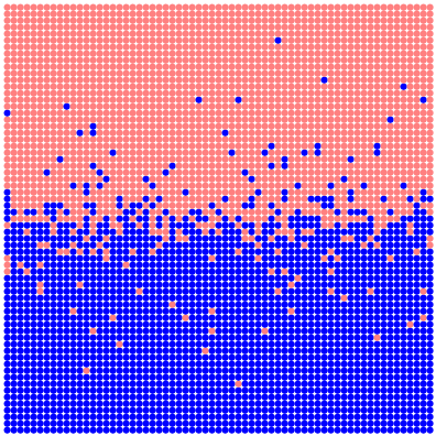
So, for example, if we use function
cf(bId0, c1, c2) = {
    c1=2: 1,
    otherwise: 2
},
we obtain the following diagram

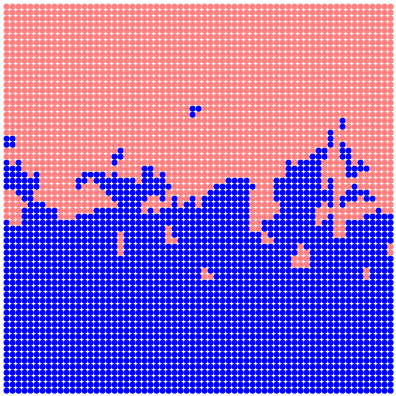
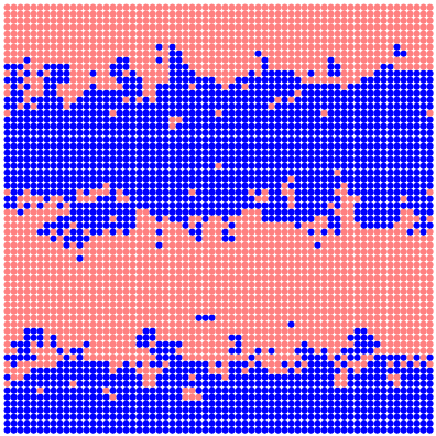
But if we reverse the points walkthrough order, then we get following satisfactory diagram with randomness and mixing of biomes.
In practice, you can remove singleton points to significantly reduce the amount of processed data, without greatly degrading the overall picture.
The mixing width is adjustable with the s parameter. For visual comparison I also give here the results for s=30.
 |
 |
The proposed function u(y) is not the only possible function here; you can use others too. So, for example, if we use cosine
we get
 |
 |
Functions dependable not only on y but also on x are also possible.
A huge advantage of this mixing method is that it can be applied to individual units of the lattice, and unit boundaries will not be noticeable in the resulting picture (squares in this case, rhombs in the project). To extend the points distribution to neighboring units, it is sufficient to fix the values at the already evaluated common boundary points.
Consideration Of Elevations
At last, we must take into account how biomes change depending on the elevation of each point of the rhombs’ lattice. A biome will change to other if the elevation exceeds a certain threshold defined by layers of global biome sequences (see the previous post). In addition, we can make some transition zone of a fixed width with mixed biomes.
For the planet Serpento, the width of this transition zone is 50-100 meters. The distribution of biomes in the transition zone is like an initial chaotic distribution of biome points above, but with elevation instead of distance, and without subsequent consolidation process (may be changed in the future!).
To be continued..