One interesting presentation of maps is the stereographic projection that projects a sphere onto a plane. In cartography it is used to map the Earth, especially near the poles, but also near other points of interest.

Here I will give an example of the stereographic projection of a part of the planet map near the north pole. For this we need two tools: GDAL and QGIS to make reprojection and see the result.

For this example I download archive of Geotiff tiles from the page of Heathcliff planet. As Wikipedia states, Geotiff is a public domain metadata standard which allows georeferencing information to be embedded within a TIFF file. The potential additional information includes map projection, coordinate systems, ellipsoids, datums, and everything else necessary to establish the exact spatial reference for the file.

For the following, we need to select only a portion of the map near the north pole. Firstly, we should run gdalbuildvrt tool from GDAL to make vrt file, which is special XML dataset composed from information about all Geotiff tiles, their positioning and sizes.

gdalbuildvrt gtiffs8.vrt <gtiffs8>/8/*/*.tif

Where <gtiffs8> is a directory in which the Geotiff tiles archive was unpacked. Next, we apply gdal_translate tool to the gtiffs8.vrt file in order to cut out a part of the map near the pole and immediately scale the resulting image.

gdal_translate -srcwin 0 10000 65536 28000 \
            -outsize 10% 10% gtiffs8.vrt pole_area.tif

Here, -srcwin option selects a subwindow from the source data set for copying based on pixel location (specific values of the pixel coordinates were determined by the size of the original data, which can be found by looking in the gtiffs8.vrt file). -outsize option sets the size of the output file as the 1% fraction of the input image size. (Output file size should be about several tens of megabytes. You can omit this option but you will get file which size is about several gigabytes.)

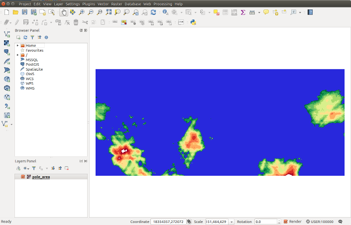
New pole_area.tif file is a Geotiff file, whose projection remained unchanged, that is the Web Mercator projection. We could use gdalwarp tool to change the projection to that we want right away, but we will use QGIS to do that and at the same time we will see the resulting image.

Click Add Raster Layer on the left palette to load pole_area.tif file into QGIS workspace.

In lower right corner of the qgis window you can see current image projection. Click on it, then Project Properties window will be opened. Choose CRS tab and check on Enable ‘on the fly’ CRS transformation if it is not already so.

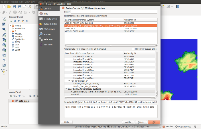
Your default projection Generated CRS (…) is to be in this window. If you select it you will see the definition of this projection at the bottom of the window. It will be something like

+proj=merc +lon_0=0 +lat_ts=0 +x_0=0 +y_0=0 +a=6378137 +b=6378137 +units=m +no_defs

For an explanation, I refer you to the proj4.org site. In the future, perhaps, I will write a separate tutorial on this topic. But now type UPS string in the Filter field and choose WGS 84 / UPS North from the list.

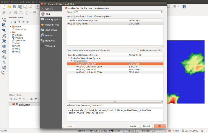
At the bottom of the window you will see the definition of this projection.

+proj=stere +lat_0=90 +lat_ts=90 +lon_0=0 +k=0.994 +x_0=2000000 +y_0=2000000 +datum=WGS84 +units=m +no_defs

Now click OK button. In the QGIS workspace you will see the stereographic projection of the north pole area.

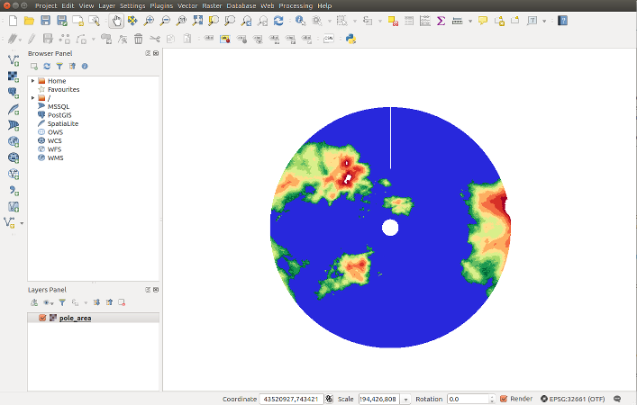
Finally, you may export the picture in any available format. If you click on the image below, you get the full size image that I exported myself.