Preliminary notes

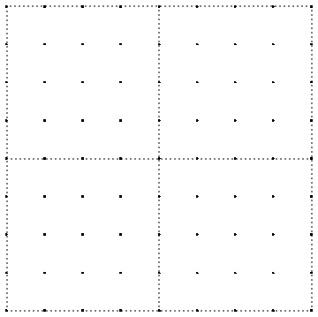
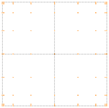
In the project it is implemented, among others, the noise functions method for the fBm surface construction. Perlin noise is the most well-known algorithm that uses noise functions for creation of random textures. First step of it can be described as follows: a special function, called basis function, is applied for a transformation of the square domain; it does this domain stretching and compressing in a certain way. See the figure below for the Perlin basis function action. (Click on figures to make them large.)

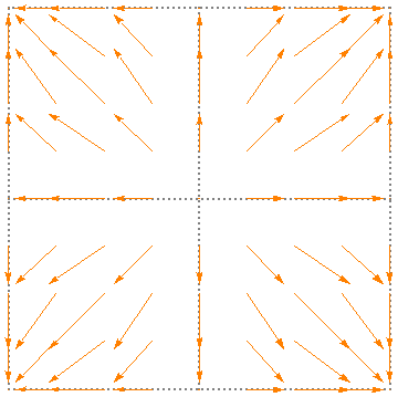The original points in the center area move away from each other accumulating near the boundaries.

Usually, the function for transform is chosen so as to provide necessary smoothness of the transformation anywhere in the square including the case of transition across the boundaries of two adjacent squares. In Perlin noise odd degree polynomials starting from third degree are used. In the figure above it is shown an example with the fifth degree polynomial.

The desired texture are a set of values at some points on the square, for example, at points of some regular square lattice. For start, some vectors a_i (i is the vertex number) are set on the vertices of the square (often random). To obtain the value at a point we do application of the basis function, after which the resulting point will be the end point of vectors b_i with start points at the square’s vertices. Then we make scalar products (a_i, b_i) and calculate average value. This value will be the desired value of the texture at the point.

Also, Perlin noise is often used to build a simple relief for isolated areas. To do this, we should create fBm surface by making multiple textures for different square sizes, which then add up with each other. Note, that for random fractals we require only statistical similarity at different levels of its scale.

If at each stage (octave) the size of squares is always reduced by r, and if the random displacements have the variance reduced by r^2H (0<H<1) compared to the previous stage, then we will get a 3D surface known as the fBm surface. This surface is an approximation to some random fractal. The value of H determine the fractal dimension. It is known that this dimension d=3-H. The larger H gives a fractal with the smaller dimension, and therefore the corresponding fBm surface will be smoother.

Note, that in practice the most convenient option is when r=1/2 (lacunarity) as suitable for simple regular lattices.

By using Perlin noise you can create separate mountains or mountain valleys. Also, it is possible to create some additional effects by post-processing, but it seems very difficult and even impossible to create complete systems of rivers and their valleys on the whole planet.

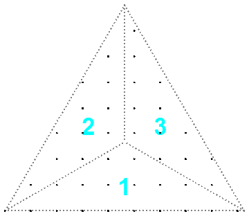
fBm on the equilateral triangle

To begin, we should choose a basis function. In reality there are infinitely many of those; we need to choose one that fits well our goal, namely, to create relief on the triangular domain. This requires compliance with certain conditions: it is desirable that the basis function is smooth inside and on edges of the triangle, and the triangle’s symmetry is also preserved when it is transformed.

For further, note that in an equilateral triangle each median is also the height and the bisector, and at their common intersection point they are divided in the ratio 2:1.

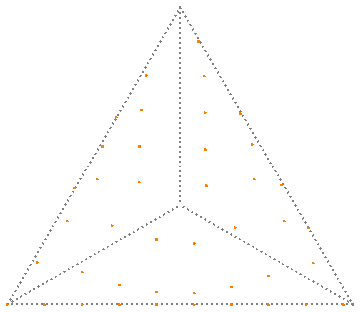
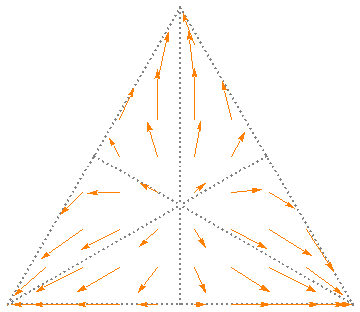
The following transformation is proposed as a basis function consisting of two steps. In the first step, a contraction of radial segments from vertices of the triangle to its medians is performed. In the second step, we do a contraction perpendicularly to the edges.

For the first step, it is convenient to divide the triangle into three parts using small segments of medians. We can unify the process by making transformation calculations only in the part 2. For calculations in the part 3 we can rotate a point around the triangle center to the part 2, or, we can do reflection in the vertical axis for a point in the part 1. Then we do the calculations as for a point in the part 2, and finally we make the inverse transformation to return to the original part.

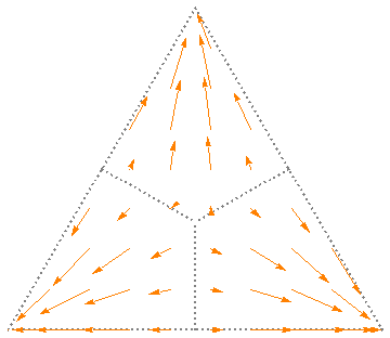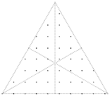
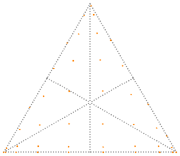
For the second step, the triangle can also be divided into three parts, but with large segments of medians. And as the working part we choose the bottom one (the part 1), where the transformation is a vertical movement of points between the medians and the bottom edge. With points in the remaining parts 2 and 3 we make the rotation around the triangle’s center, then we do the transformation as with a point in part 1, and then the reverse rotation.

By successively performing all transformations we will get the basis function action as on the following figure.

You may ask, if is it possible in practice to use more simple Perlin noise in all cases. I would answer in this way. In all those cases when a texture is created for any bounded part of the plane, then Perlin noise will be fine. But, if you are dealing with an enclosed 3D surface, which can be divided into equal equilateral triangles (triangulation), then it is natural to use a method similar to the one proposed, because it allows you to cover the entire surface with the texture without visible stitches. This is exactly what is required in this project in order to be able to construct the fBm surface on the entire planet’s sphere without discontinuities. The surfaces of tree regular polyhedra, for another example, allow triangulation with equal equilateral triangles.

The basis function code for the equilateral triangular domain

Here I will digress a little from the usual way of narration in this blog, where I try to give a minimum of formulas or code, more limited to simple reasoning (I hope that it have always been clear, despite the shortcomings of fluency in my English). Moreover, I do not know whether there is somewhere a similar approach in the public domain.

The code below is a slightly modified copy-paste from the project’s code. Like most of the project it is written in Haskell, but the code of computational parts, I think, will be clear to anyone knowing any common programming language. Therefore, I did not do the translation to pseudocode. Anyone who is interested can freely use it, improve it, rewrite it to other languages, and distribute.

Just in case, I will explain some of the Haskell features that can be confusing in this code.

• In records like (tA p-abs x) * tanPiD3 p, you need to take into account that grabbing function’s arguments is an operation with a higher priority than arithmetic operations; in the most other languages this may be equivalent to (tA(p)-abs(x)) * tanPiD3(p).
• Haskell is a language where lazy calculations are used by default. Where it seems to you that unnecessary calculations are being made, you are wrong.
• Reader monad. The value written to it is obtained by the operation p<-ask. The monads in Haskell are operations with a certain context; in this case we use Reader monad to transfer pre-calculated constant values to the functions.

First comes the module header and data type definitions. In the calculations we consider the length of the triangle edge a=1. The origin of Cartesian coordinate system is in the center of the triangle’s bottom edge. The vertices have coordinates (-0.5, 0), (0.5, 0), (0, tY p)≈(0, 0.866)

module Fbm.Triangle.Basis where

import Control.Monad.Reader

--| Data type for an arbitrary triangle point
data (RealFloat fv) => TPoint fv = TPoint !fv !fv
        deriving (Show, Eq)

--| Data type for a record of constant values
data (RealFloat fv) => TParams fv = TParams
        { tA        :: fv
        , tCY       :: fv
        , tY        :: fv
        , tanPiD6   :: fv
        , tanPiD3   :: fv
        }

-- | Triangle part
type TPart = Int

--| Calculates the constant values, which we need further.
calcTParams
    :: RealFloat fv
    => TParams fv
calcTParams = tPrms where
    a = 1.0
    tanPiD6' = tan (pi/6)
    tPrms = TParams
        { tA        = a / 2
        , tCY       = a * tanPiD6' / 2 -- a * tan (pi/6) / 2
        , tY        = a / tanPiD6' / 2 -- a * tan (pi/3) / 2
        , tanPiD6   = tanPiD6'
        , tanPiD3   = 1/tanPiD6' -- tan (pi/3)
        }

{-| Makes transformed values. It allows to choose one of several transformations. It also makes normalization of the variable t over the full length of the interval s of the function domain. In implementations of the Perlin noise algorithm this procedure is often called 'lerp'.
-}
interp
    :: RealFloat fv
    => Int
    -> fv
    -> fv
    -> fv
interp p t s = if t<=0 then 0 else val where
    t' = t/s
    val
      | p==7    = 35*(t'**4) - 84*(t'**5) + 70*(t'**6) - 20*(t'**7)
      | p==5    = 10*(t'**3) - 15*(t'**4) + 6*(t'**5)
      | p==3    = 3*(t'**2) - 2*(t'**3)
      | p==1    = t'
      | otherwise = error $ "interp: undefined function for power "++show p

--| Checks that a point is in the triangle. Not called in the functions of this module.
checkTPoint
    :: RealFloat fv
    => TPoint fv
    -> Reader (TParams fv) (Either String (TPoint fv))
checkTPoint tp0@(TPoint x y) = do
    p <- ask
    let tp1
          | abs(x)>tA p                 = Left "TPoint: invalid x"
          | y<0 || y>tY p               = Left "TPoint: invalid y"
          | y>(tA p-abs x)*tanPiD3 p    = Left "TPoint: out of triangle"
          | otherwise                   = Right tp0
    return tp1

--| Gets the part of the triangle, which contains a point for the first transformation.
getTrianglePart1
    :: (RealFloat fv, Show fv)
    => TPoint fv
    -> Reader (TParams fv) TPart
getTrianglePart1 (TPoint x y) = do
    p <- ask
    let part
          | y<=tCY p - tCY p/tA p*x && x<0  = 1
          | y<=tCY p + tCY p/tA p*x         = 2
          | otherwise                       = 3
    return part

-- | Gets the part of the triangle, which contains a point for the second transformation.
getTrianglePart2
    :: (RealFloat fv, Show fv)
    => TPoint fv
    -> Reader (TParams fv) TPart
getTrianglePart2 (TPoint x y) = do
    p <- ask
    let sn = negate (signum x)
        part
          | y<=tCY p/tA p*(sn*x+tA p)   = 1
          | x<=0                        = 2
          | otherwise                   = 3
    return part

-- | Rotation
rotateC
    :: RealFloat fv
    => fv
    -> TPoint fv
    -> Reader (TParams fv) (TPoint fv)
rotateC phi (TPoint x0 y0) = do
    p <- ask
    let x1 = x0*cos phi - (y0-tCY p)*sin phi
        y1 = x0*sin phi + (y0-tCY p)*cos phi + tCY p
    return $ TPoint x1 y1

-- | Reflection
flipX
    :: RealFloat fv
    => TPoint fv
    -> Reader (TParams fv) (TPoint fv)
flipX (TPoint x y) = return $ TPoint (-x) y

{-| The first step of the transformations. 'smooth' procedure makes the correction
to the transform to weaken displacements for long domains; this slightly improves
the final result.
-}
interpT1
    :: (RealFloat fv, Show fv)
    => InterFPower
    -> TPoint fv
    -> Reader (TParams fv) (TPoint fv)
interpT1 ifp tp0@(TPoint x0 y0) = do
    p <- ask
    let smooth (TPoint x y, c) = TPoint (x0+c*(x-x0)) (y0+c*(y-y0))
        tanA = y0/(tA p - x0)
        cosA = cos (atan tanA)
        xS = if tanA>tanPiD6 p
                then (tA p*tanA - tCY p) / (tanA + tCY p/tA p)
                else 0
        lL = (tA p-xS)/cosA
        l0 = (tA p-x0)/cosA
        l1 = 2*lL * interp ifp l0 (2*lL)
        x1 = tA p - l1*cosA
        y1 = (tA p-x1) * tanA
    if x0>=tA p || isNaN tanA
        then return tp0
        else return $ smooth (TPoint x1 y1, (tA p/lL)**0.5)

--| The second step of the transformations.
interpT2
    :: (RealFloat fv, Show fv)
    => InterFPower
    -> TPoint fv
    -> Reader (TParams fv) (TPoint fv)
interpT2 ifp tp0@(TPoint x0 y0) = do
    p <- ask
    let y0' = if y0<0 then 0 else y0
        lL = tanPiD6 p * (tA p - abs x0)
        y1 = 2*lL * interp ifp y0' (2*lL)
    if abs x0>=tA p
        then return tp0
        else return $ TPoint x0 y1

{-| Calls for the basis function action. After the first transformation is done, the second transformation is applied to the resulting point.
-}
interpT
    :: (RealFloat fv, Show fv)
    => InterFPower
    -> InterFPower
    -> TPoint fv
    -> Reader (TParams fv) (TPoint fv)
interpT ifp1 ifp2 tp0 = do
    let an = 2*pi/3
        tr1 tp = do
            pt <- getTrianglePart1 tp
            let tp'
                  | pt==1 = flipX tp >>= interpT1 ifp1 >>= flipX
                  | pt==2 = interpT1 ifp1 tp
                  | pt==3 = rotateC (-an) tp >>= interpT1 ifp1 >>= rotateC an
                  | otherwise = error $ "interpT: invalid triangle part 1"
            tp'
        tr2 tp = do
            pt <- getTrianglePart2 tp
            let tp'
                  | pt==1 = interpT2 ifp2 tp
                  | pt==2 = rotateC an tp >>= interpT2 ifp2 >>= rotateC (-an)
                  | pt==3 = rotateC (-an) tp >>= interpT2 ifp2 >>= rotateC an
                  | otherwise = error $ "interpT: invalid triangle part 2"
            tp'
    return tp0 >>= tr1 >>= tr2

This completes the module.

Let’s see how we can use the main ‘interpT’ procedure. This require a few more procedures.

import Fbm.Triangle.Basis

--| Dot multiplication
dot
    :: RealFrac fv
    => (fv, fv)
    -> (fv, fv)
    -> fv
dot (x1, y1) (x2, y2) =
    x1*x2 + y1*y2

{-| Makes an average of scalar product results (v1, v2, v3), taking into account the distances to the vertices of the triangle from the given point.
-}
avgT
    :: (RealFloat fv, Show fv)
    => (fv, fv, fv)
    -> TPoint fv
    -> Reader (TParams fv) fv
avgT (v1, v2, v3) (TPoint x y) = do
    p <- ask
    let yP2 = y**2
        lx = (tY p-y) * tanPiD6 p
        d2 = sqrt ((x-0.5)**2+yP2)
        d2min = sqrt ((lx-0.5)**2+yP2)
        d2max = sqrt ((lx+0.5)**2+yP2)
        u1' = (d2-d2min) / (d2max-d2min)
        (u1, u2)
          | u1'>1   = (1, 0)
          | u1'<0   = (0, 1)
          | otherwise   = (u1', 1-u1')
        w = y/tY p
        val = w * v3 + (1-w) * (u1*v1+u2*v2)
    return $ if y>=tY p || isNaN val then v3 else val

{-| Calculates the desired value of the texture in a point with vectors (vc1, vc2, vc3) set in the corresponding triangle's vertices.
-}
noiseT
    :: (RealFloat fv, Show fv)
    => ((fv, fv), (fv, fv), (fv, fv))
    -> TPoint fv
    -> Reader (TParams fv) fv
noiseT (vc1, vc2, vc3) tp0 = do
    p <- ask
    tp@(TPoint x y) <- interpT 7 3 tp0    
    let y3 = y'-tY p
        v1 = dot (x+0.5, y) vc1
        v2 = dot (x-0.5, y) vc2
        v3 = dot (x, y3) vc3
    avgT (v1, v2, v3) tp

Using in the project

The following figure is an example of this method usage. Each rhomb from the covering of the planet’s sphere can be divided into two equilateral triangles: the upper one and the lower one. Here, it is applied the equivalent of ‘noiseT’ procedure to the points of the regular triangular lattice. To match textures defined on adjacent triangles we must always require to set the same vectors vc in joint vertices. (Click on the figure to make it larger.)

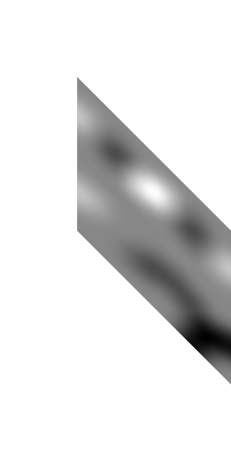
ifp1=7 is used for the first step, and ifp2=3 for the second. This is the case that turned out to be optimal. After summation of 7 texture layers (octaves) we get fBm image as in the following figure. (Click on the figure to make it larger.)

*The green dotted lines are the borders of rhombs.

To be continued..