This is the final post of this topic. Here we turn our eyes to how the smallest relief details can be created. In one of the previous posts we have learned about base heights surface. We discovered that all the riverbeds lie on that surface, but it is devoid of small relief details. For these we should create a special layer, which is called local heights grid. Perhaps more accurately, it should be called terrain layer or hills layer.

Of course, in these posts, I mean not solid surfaces, but grids of discrete points that can be ‘visually supplemented’ to a continuous surface.

The local heights grid is built at the same points as the base heights grid. It determine the specific view of mountain regions and lowlands. We must consider several factors when creating it. Firstly, the riverbeds must remain in their place, that is, the values at river points should be equal to zero. Secondly, in areas where base heights are large the local height values should also be preferably greater, which corresponds to larger differences in elevation on the higher grounds. Last rule for the Earth is not absolute, but at the moment I follow it in the planets creation.

I use the old good fBm surface approach but with a certain transformation. It can be interpreted as modulation of the fBm surface by a certain function. For clarity, I will initially resort to a 2D analogy, which can be interpreted as a vertical section of some relief.

As can be seen on the Earth’s surface, rivers in the plains and in the mountains have different valley profiles. In plains the terrain heights rises slowly, and in the mountains heights get up steeply followed by rugged terrain area.

Hill function

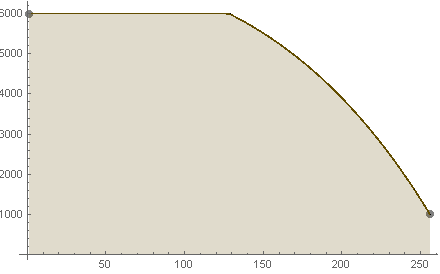
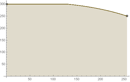
To specify diversity of the river valley forms, I use a special distribution function. It determines the maximum possible value of the terrain layer at a point of the rhombs’ local lattice. This function (hill function) defined as this.

hillV(d, sc) = sc*(d^p-1)/m, where m = r^p-1.

The power p>-1; d is the distance to the nearest riverbed (d>=1); r is the maximum possible distance from any point to any riverbed; sc is the scaling value, which in turn can depend on the base height at the point. Graphics of hill function for various power p are shown in the following figure.

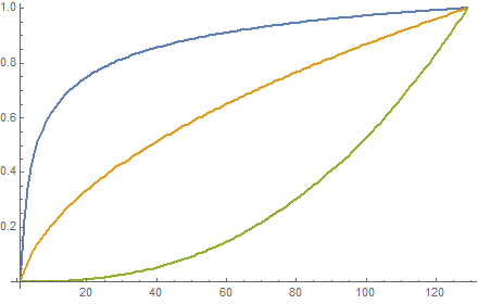
(blue: p=-0.25, yellow: p=0.5, green: p=2.5)

We should use lesser powers for lowland valleys and greater powers for mountainous ones. Thus, power p should be a monotonic function of the base height h. On the planet Serpento it is linear from -0.9 to 0.4, and these are rather extreme values!

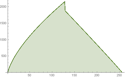
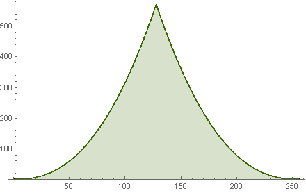
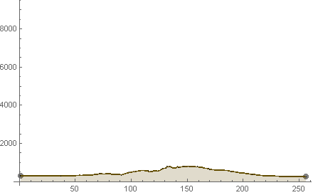
At each lattice point of a rhomb we calculate the value of this function. For a 2D case the result is shown on the following figure.

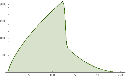
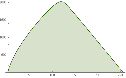
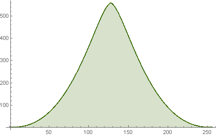
To refine the resulting curve we can use smoothing. If we use simple averaging over neighboring points, we get the first figure below. But we can get better result like in the second figure in a different way.

For that, firstly, we should sort the rhomb points in descending order of hillV function values evaluated at them, and then we should calculate the new values successively using the next formula.

v1 = (maxV−minV)/k + minV.

Here, minV and maxV are the minimum and the maximum values at the neighborhood points. k>=2 is a variable that must monotonously decrease from the maximum value mK in points mostly distant from any riverbed to 2 at riverbed points. In the figure above k decreases linearly, k=10 at the central points and k=2 at the edges.

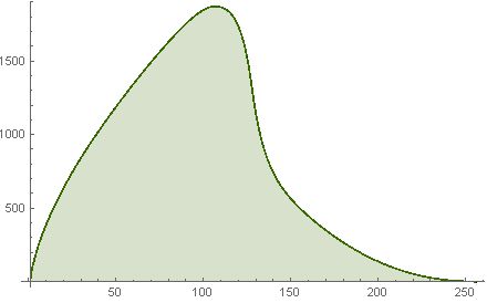
Then again we go through all the points and set the other new values in them using the formula.

v2 = maxV − (maxV−minV)/k,

where k behaves similar, but may have a different mK in general case.

The distribution of v2 values is presented in the second figure above. Further, when we will talk about smoothing we will mean just such a process of calculating v2 values.

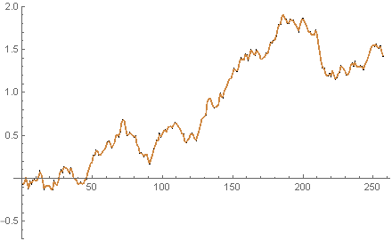
Now let’s move on to the modulation itself. We get the fBm surface (for example, by the way shown in the previous post) and its values are multiplied by the smoothed values of the hill function at the same points.

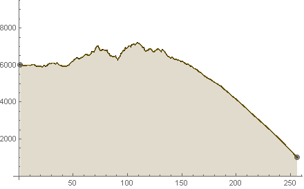
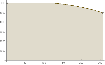
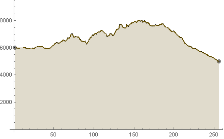
Suppose, for example, that we have obtained 2D fBm curve as in the following figure.

Adding up the values of the modulation result’s curve (the first figure below) with the curve of the base heights (the second figure) we get the final relief (the third figure).

In order to better understand the result, I give here the results of two other cases for different heights of two riverbeds, while using the same fBm curve.

Case 2. Both rivers are at high elevation.

Case 3. Both rivers are at low elevation.

3D model of modulation surface

It should be clearer now what happens in the 3D case. Just as for the base heights surface, for simple model we choose several points with zero value at them, which corresponds to the points with fixed values in the riverbeds.

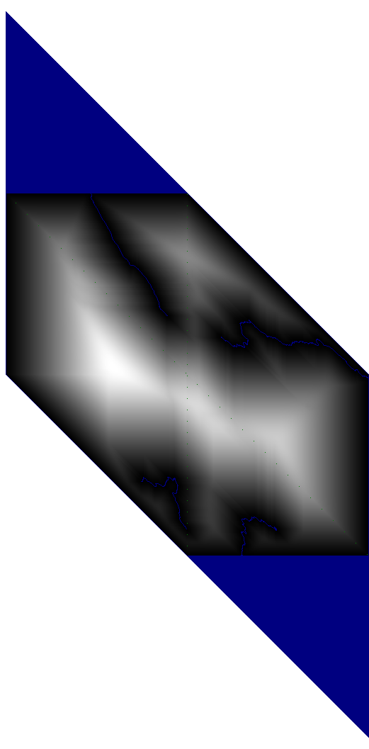
The first diagram is the values of the 3D hill function.

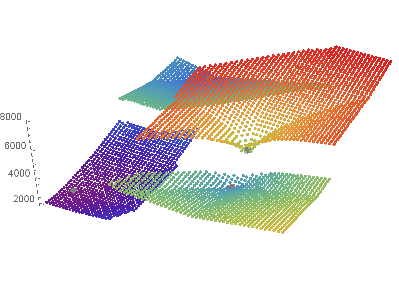
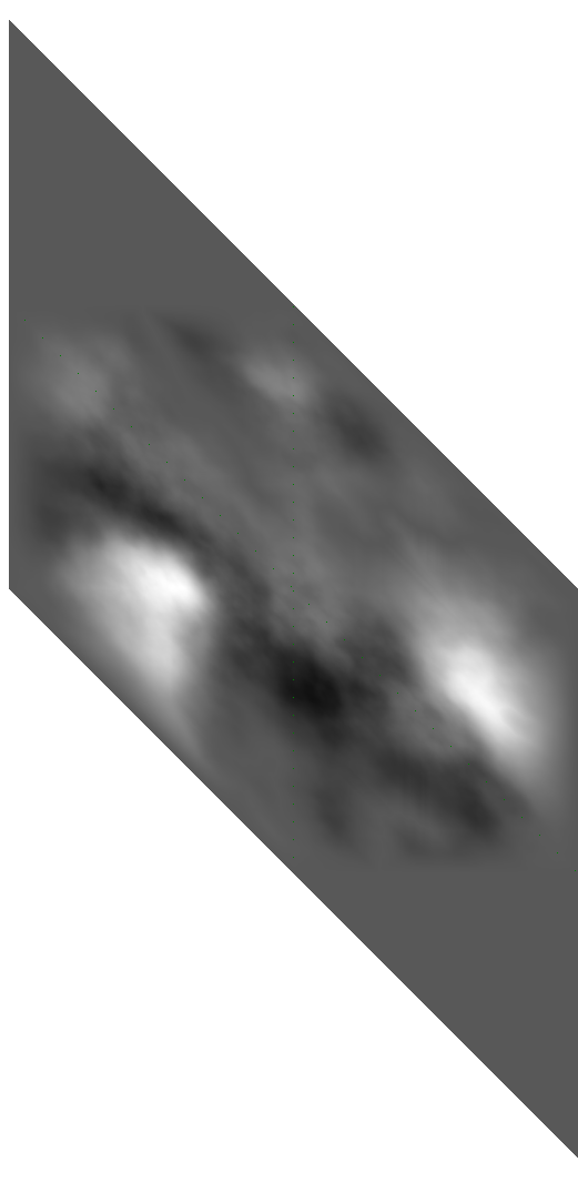
Next, we calculate the v1 and v2 values using the same formulas. But now we need to sort additionally the points by v1 values before calculating v2 values.

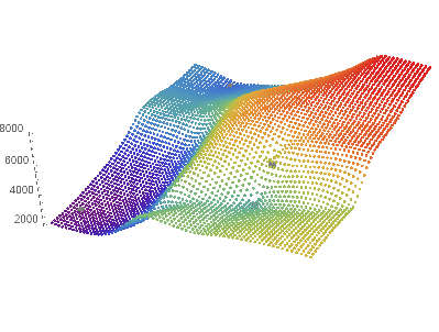
As we can see, the surface has noticeable gaps. We do v1 and v2 calculations again with sorting at every step and with lower mK values. As the result we get a smoother surface.

Thus, by an iterative process, we can improve the smoothness of the modulation surface.

As final step, we can additionally apply smoothing over the points’ neighborhood and get the acceptable result for the modulation surface.

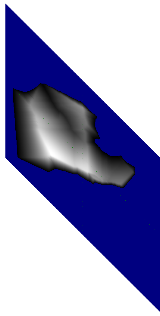
Using in the project

Here is an example of the modulation surface for one island on a test planet (first figure). After applying it to the fBm surface (in the project the fBm values can be negative) we get second figure.

As an interesting intermediate result we may add the modulation surface values directly to the base heights (first figure). But let’s do it right, and at the last stage we add together the values of the base heights grid and the modulated fBm surface (second figure).

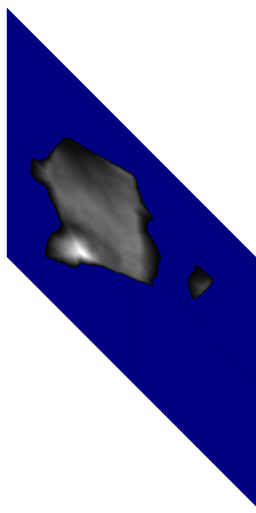We have a hilly island with a single mountain on its edge and with a satellite island. Depression for the bed of a single river clearly visible. Also, additional work has been done here to make the sea coast more steep, but this is a separate topic.

Although described smoothing process was used to create above figures, so far simple averaging over neighbors are used for creation of whole planets. It was particularly used to create the Serpento planet.

The smoothing method presented here has such a feature that the new values are highly dependent on their environment and direct application to individual rhombs can lead to very noticeable effects at the rhombs’ edges. Currently, the project implements an iterative process only for each rhomb individually, and it should be redone for a process in which a some set of close rhombs is involved.

Also, the issue of the direct participation of riverbed points in smoothing process remains open, if we allow this, the river sources will be raised rather than deepened as they are now. But this can also be satisfactorily resolved only after the correct implementation of the iterative smoothing process.